
I have written about how to run the ANOVA test in my previous post Analysis of Variance ANOVA using R. We analyzed the salary difference between different level of education.
For ease of (my!) understanding, I would take the same data set in this post as well. So here is the same data set.
> sal
   id gender      educ  Designation Level Salary Last.drawn.salary Pre..Exp Ratings.by.interviewer
1   1 female        UG  Jr Engineer   JLM  10000              1000        3                      4
2   2   male DOCTORATE     Chairman   TLM 100000            100000       20                      4
3   3   male   DIPLOMA        Jr HR   JLM   6000              6000        1                      3
4   4   male        PG     Engineer   MLM  15000             15000        7                      2
5   5 female        PG  Sr Engineer   MLM  25000             25000       12                      4
6   6   male   DIPLOMA  Jr Engineer   JLM   6000              8000        1                      1
7   7   male   DIPLOMA Jr Associate   JLM   8000              8000        2                      4
8   8 female        PG     Engineer   MLM  13000             13000        7                      3
9   9 female        PG     Engineer   MLM  14000             14000        7                      2
10 10 female        PG     Engineer   MLM  16000             16000        8                      4
11 11 female        UG  Jr Engineer   JLM  10000              1000        3                      4
12 12   male DOCTORATE     Chairman   TLM 100000            100000       20                      4
13 13   male   DIPLOMA        Jr HR   JLM   6000              6000        1                      3
14 14   male        PG     Engineer   MLM  15000             15000        7                      2
15 15 female        PG  Sr Engineer   MLM  25000             25000       12                      4
16 16   male   DIPLOMA  Jr Engineer   JLM   6000              8000        1                      1
17 17   male   DIPLOMA Jr Associate   JLM   8000              8000        2                      4
18 18 female        PG     Engineer   MLM  13000             13000        7                      3
19 19 female        PG     Engineer   MLM  14000             14000        7                      2
20 20 female        PG     Engineer   MLM  16000             16000        8                      4
21 21 female        PG  Sr Engineer   MLM  25000             25000       12                      4
22 22   male   DIPLOMA  Jr Engineer   JLM   6000              8000        1                      1
23 23   male   DIPLOMA Jr Associate   JLM   8000              8000        2                      4
24 24 female        PG     Engineer   MLM  13000             13000        7                      3
25 25 female        PG     Engineer   MLM  14000             14000        7                      2
26 26 female        PG     Engineer   MLM  16000             16000        8                      4
27 27 female        UG  Jr Engineer   JLM  10000              1000        3                      4
28 28   male DOCTORATE     Chairman   TLM 100000            100000       20                      4
29 29   male   DIPLOMA        Jr HR   JLM   6000              6000        1                      3
30 30   male        PG     Engineer   MLM  15000             15000        7                      2
31 31 female        PG  Sr Engineer   MLM  25000             25000       12                      4
32 32 female        PG  Sr Engineer   MLM  25000             25000       12                      4
33 33   male   DIPLOMA  Jr Engineer   JLM   6000              8000        1                      1
34 34   male   DIPLOMA Jr Associate   JLM   8000              8000        2                      4
35 35 female        PG     Engineer   MLM  13000             13000        7                      3
36 36 female        PG     Engineer   MLM  14000             14000        7                      2
37 37 female        PG     Engineer   MLM  16000             16000        8                      4
38 38 female        UG  Jr Engineer   JLM  10000              1000        3                      4
39 39   male DOCTORATE     Chairman   TLM 100000            100000       20                      4
40 40   male   DIPLOMA        Jr HR   JLM   6000              6000        1                      3
41 41   male        PG     Engineer   MLM  15000             15000        7                      2
42 42 female        PG  Sr Engineer   MLM  25000             25000       12                      4
43 43   male   DIPLOMA  Jr Engineer   JLM   6000              8000        1                      1
44 44   male   DIPLOMA Jr Associate   JLM   8000              8000        2                      4
45 45 female        PG     Engineer   MLM  13000             13000        7                      3
46 46 female        PG     Engineer   MLM  16000             16000        8                      4
47 47 female        UG  Jr Engineer   JLM  10000              1000        3                      4
48 48   male DOCTORATE     Chairman   TLM 100000            100000       20                      4
49 49   male   DIPLOMA        Jr HR   JLM   6000              6000        1                      3
50 50   male        PG     Engineer   MLM  15000             15000        7                      2
We have already executed ANOVA test. Following is the output.
> aov1 <-aov(Salary~educ, data=sal)
> aov1
Call:
   aov(formula = Salary ~ educ, data = sal)

Terms:
                       educ   Residuals
Sum of Squares  35270186667   538293333
Deg. of Freedom           3          46

Residual standard error: 3420.823
Estimated effects may be unbalanced
> summary(aov1)
            Df    Sum Sq   Mean Sq F value Pr(>F)
educ         3 3.527e+10 1.176e+10    1005 <2e-16 ***
Residuals   46 5.383e+08 1.170e+07
---
Signif. codes:  0 ‘***’ 0.001 ‘**’ 0.01 ‘*’ 0.05 ‘.’ 0.1 ‘ ’ 1
Variance between groups
What we get above is the overall significant difference between DV (salary) and IV (Education)
To compare the difference between the group, we use Post hoc test. We shall use TukeyHSD() for this. We need to go for this approach, only if the anova is significant. If anova is not significant, there is no need for posthoc.
We’d see how to run get the variances across the groups in this post.
> tukey <- TukeyHSD(aov1)
> tukey
  Tukey multiple comparisons of means
    95% family-wise confidence level

Fit: aov(formula = Salary ~ educ, data = sal)

$educ
                        diff        lwr        upr     p adj
DOCTORATE-DIPLOMA  93333.333  88624.720  98041.947 0.0000000
PG-DIPLOMA         10373.333   7395.345  13351.322 0.0000000
UG-DIPLOMA          3333.333  -1375.280   8041.947 0.2477298
PG-DOCTORATE      -82960.000 -87426.983 -78493.017 0.0000000
UG-DOCTORATE      -90000.000 -95766.850 -84233.150 0.0000000
UG-PG              -7040.000 -11506.983  -2573.017 0.0006777
- diff – mean difference between education level
- lwr – lower mean
- upr – upper mean
If signs between lwr and upr are same, irrelevant of + or -, that denotes significant difference.
When you compare diploma (lower degree) with doctorate (higher degree), the difference would be +ve and vice versa. If you just want to see the difference, + or – is not significant.
Let’s plot this in a graph.
> plot(tukey)
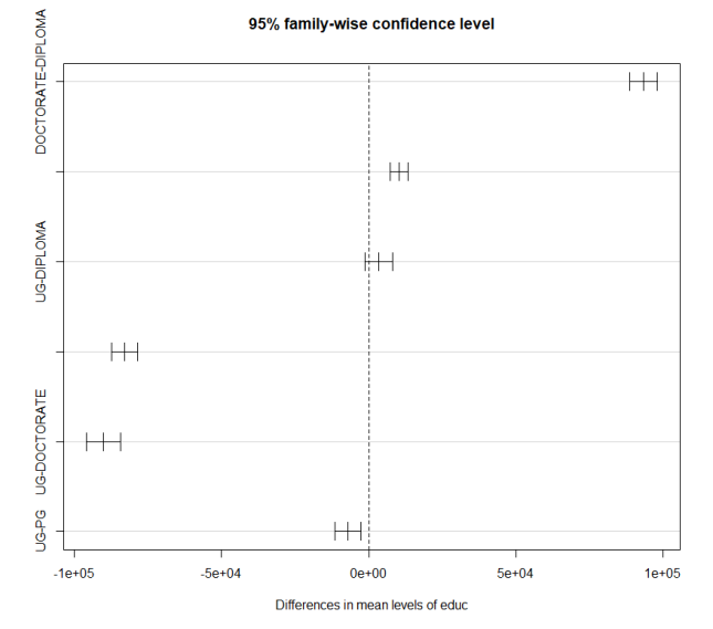
0 is the mid point. So, anything near 0 do not have significant difference.
From the top, first plot is for the comparison between DOCTORATE-DIPLOMA. You would see a high positive difference. If you see the plot for UG-DOCTORATE, is it second highest difference, but this is negative difference. Anything near 0 like UG-DIPLOMA, does not have significant difference.
ANOVA between multiple variables
We received a new data set from company now, which has a new column Loan.deducation. Last.drawn.salary changes with respect to his loans.
> sal <- read.csv("sal.csv")
> head(sal)
  id gender      educ Designation Level Salary Loan.deduction Last.drawn.salary Pre..Exp Ratings.by.interviewer
1  1 female        UG Jr Engineer   JLM  10000        5901.74           4098.26        3                      4
2  2   male DOCTORATE    Chairman   TLM 100000        4247.31          95752.69       20                      4
3  3   male   DIPLOMA       Jr HR   JLM   6000        3895.76           2104.24        1                      3
4  4   male        PG    Engineer   MLM  15000        9108.36           5891.64        7                      2
5  5 female        PG Sr Engineer   MLM  25000        4269.39          20730.61       12                      4
6  6   male   DIPLOMA Jr Engineer   JLM   6000        4137.31           1862.69        1                      1
Company wants to see the differences among Salary (column 6), Loan.deduction (column 7) and Last.drawn.salary (column 8). We combine apply and anova as given below.
> aovset <- apply(sal[,6:8], 2, function(x)aov(x~educ, data = sal))
- sal[,6:8] takes all rows of columns 6, 7 and 8
- aov is our function
Following is the variance between education and Last.drawn.salary.
> summary(aovset$Last.drawn.salary)
            Df    Sum Sq   Mean Sq F value Pr(>F)
educ         3 3.342e+10 1.114e+10   674.2 <2e-16 ***
Residuals   46 7.602e+08 1.653e+07
---
Signif. codes:  0 ‘***’ 0.001 ‘**’ 0.01 ‘*’ 0.05 ‘.’ 0.1 ‘ ’ 1
F value is 674, which means, the change is significant. Following would be more interesting.
> summary(aovset$Loan.deduction)
            Df    Sum Sq Mean Sq F value Pr(>F)
educ         3  25577616 8525872    1.14  0.343
Residuals   46 343898395 7476052
F value for Loan.deduction is lesser than 4. So, there is no change in the deductions between different education level.
See you in another interesting post.

Pingback: Regression testing in R | JavaShine